This blog post is currently at Embedded Related, so go there and read it !
Blog
When a Mongoose met a MicroPython
This blog post is currently at Embedded Related, so go there and read it !
“Bellegram”, a DIY wireless doorbell
This blog post is currently at Embedded Related, so go there and read it !
https://www.embeddedrelated.com/showarticle/1540.php
On hardware state machines: How to write a simple MAC controller using the RP2040 PIOs
This article has moved to my blog in Embedded Related, here
Remote development with MQTT and a little help from my friend
Not too long ago, my friend Diego contacted me to solve a technical issue for an art event. He had this idea of a neon sign, well, two actually, the message was split in half with a strong change in meaning and he wanted the second half to activate once a visitor was actually observing the photos that carried other dimension to the message.
We talked for a while and ruled out motion sensors, people stay still while watching photos. I wanted to try those new time-of-flight distance measurement chips, but their field of view was extremely narrow and we needed to cover a 4-meter wide distance two meters away from the piece of art, and we couldn’t do anything to the lateral walls…
As not long ago I’ve been designing a liquid level measurement device based on Acconeer‘s radar chips, I suggested we could use two of them to cover the area.
Under “normal” circumstances I would design something specific with a microcontroller, develop in C, and rely on Mongoose or Mongoose-OS if I needed comms. We had little more than a month to do this, I was busy with other projects, the event would take place in Miami, I live several thousands of miles south, and my friend is an artist… Diego is computer literate, we met decades ago at the Amiga forums in the Fido network (yes, we used dial-up modems and sent already written messages), but I needed to be able to calibrate the radars and make corrections to the software from my place.
I suggested to use a Raspberry Pi with WiFi, a relay board to control the lights, and two radar modules with USB connection. Diego bought them all and soon had them connected at his place; he also added a subscription to VNC so we both were able to access the RPi behind firewalls.
I chose Python for the software, that would allow me to try things on the fly and modify at will with remote access. I wrote a couple of mock libraries and developed the software on my computer (I didn’t have a Raspberry Pi), I already had one sensor and the manufacturer library provided simulation for the second one.
One design choice was to use Paho-MQTT for communications. Not only would this device report any activity (that we could later analyze to take information on visitor activities), but I needed to be able to see what the radars were seeing in order to properly configure their gain and sensitivity.
Once developed, the software was uploaded to a Github repository, then I connected to the RasPi via VNC and cloned the repo there. The radar modules came without a firmware loaded, so I uploaded it to the RPi along with the microcontroller flashing tool, asked Diego to press the proper buttons (we communicated through Whatsapp) on the modules and flashed them. Wrote a small piece of code so he could test the relays, and everything was ready for the hard part.
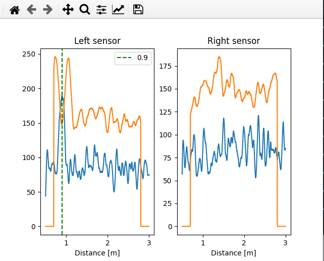
The Python program reads both sensors raw data and using Acconeer Exploration Tool (in algorithm mode) processes five readings per second and measures the distance to the closest peak detected by a CFAR algorithm. If that peak is at the desired distance range, which we estimated at a visitor typical viewing distance from 60cm to 2.5m, the program activates the relay that turns on the complementary neon sign (though they actually are LED signs in neon color…) and keeps it on for 10 seconds after all activity ceases. Every action, and no action for 1 minute, is published on a well-known (for us) MQTT topic on HiveMQ’s free broker. We could then know if the device is working by just subscribing to that topic. Paho-MQTT runs as a separate thread, the whole program in the main thread.
Besides that, I also added a small set of RPC calls, the device listens on a topic and I, from my lab, publish questions asking the status and providing a rendezvous point (the topic where the device will publish its response) and get the average data, the threshold, and any detection, inside a JSON object. This is done with a separate Python program, also based on Paho, running on my workstation. This program then uses pyplot (I’m used to MATLAB so…) to graph the readings and provide me with an idea of what is going on in Miami.
The hard part was finding the sweet spot of both sensor orientation and gain/sensitivity to achieve proper human detection with minimum false positives. We humans are not good microwave reflectors so the SNR was really poor. We asked but the art gallery personnel said dressing the visitors in full metal jacket was not an option, so Diego would walk the area phone in hand, texting me via Whatsapp, while I, 7000Km away, would watch the graphs and tweak gain and sensitivity.
Happily, we were able to get this device working OK right on time, and my friend enjoyed the reception at the art gallery while I grabbed a beer at home.
MQTT over TLS-PSK with the ESP32 and Mongoose-OS
This article is an extension to this one; I suggest you read it first.
Should you need more information on the MQTT client and using it with no TLS, read this article. For a bit more on TLS, this one.
TLS-PSK
There is a simpler solution to using full-blown TLS as we’ve seen on our first article; instead of using certificates, broker and connecting device can have a pre-shared key (PSK).
The connection process is similar, but in this case, instead of validating certificates and generating a derived key, the process starts with the pre-shared key. Depending on the scheme being used, demanding Public Key Cryptography operations can be avoided, and key management logistics can be a bit simpler, plus, we don’t need a CA (Certification Authority) anymore.
Even though there are currently three different ways to work, where one of these allows broker validation using certificates and device validation using a PSK, we’ve only tested the simplest form.
Configuration
Let’s configure the ESP32 running Mongoose-OS to use TLS-PSK.
libs:
  - origin: https://github.com/mongoose-os-libs/mqtt  # Include the MQTT client
config_schema:
  - ["mqtt.enable", true]             # Enable the MQTT client
  - ["mqtt.server", "address:port"]   # Broker IP address (and port)
  - ["mqtt.ssl_psk_identity", "bob"]  # identity to use for our key
  - ["mqtt.ssl_psk_key", "000000000000000000000000deadbeef"] # key AES-128 (or 256)
  - ["mqtt.ssl_cipher_suites", "TLS-PSK-WITH-AES-128-CCM-8:TLS-PSK-WITH-AES-128-GCM-SHA256:TLS-ECDHE-PSK-WITH-AES-128-CBC-SHA256:TLS-PSK-WITH-AES-128-CBC-SHA"] # cipher suites
The most common port for MQTT over TLS-PSK is 8883. The broker can also request we send a username and password, though the usual stuff is to configure it to take advantage of the identity we’re already sending, as we did on these tests (example below).
Regarding cipher suites, we need to provide a set of cryptographic schemes supported by our device, and at least one of them must also be supported by the broker. This is a mandatory parameter, otherwise our device won’t announce any TLS-PSK compatible cipher suite and TLS connection will not take place. Usually we negotiate this with the broker admins.
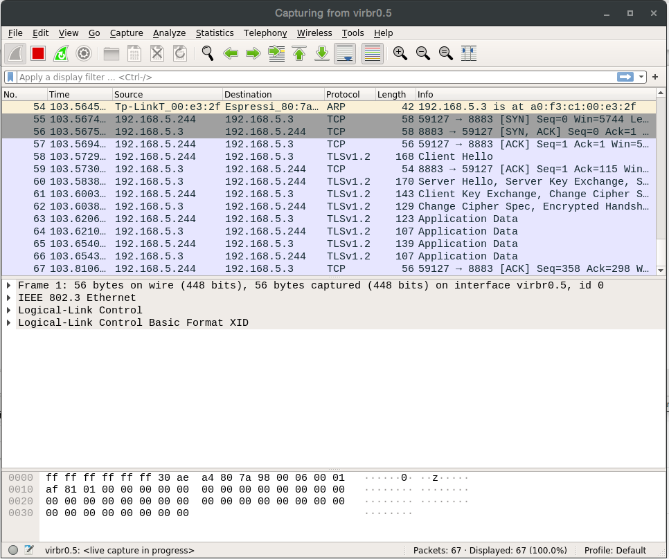
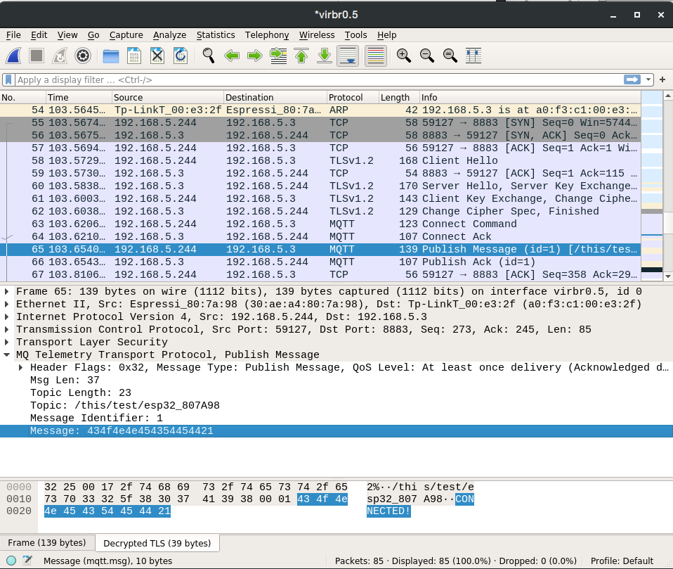
When starting the TLS connection, the device sends its supported cipher suites in its ClientHello message; the broker then chooses one that it supports and indicates this on its ServerHello message. As we’ve obtained this list by analyzing the source code, we decided to publish it here so it can be of use. In our particular case, only one of the device cipher suites was also supported by the broker: TLS-PSK-WITH-AES-128-CCM-8. The start handshake with these messages can be seen at the Wireshark snapshot below.
Finally, our pre-shared key (PSK, parameter ssl_psk_key) must be a 128-bit (16-byte) quantity for AES-128 suites and a 256-bit (32-byte) quantity for AES-256 suites.
Operation
At startup, we’ll watch the log and check if everything is going on as it should, or catch any possible errors. In this sad case, it is pretty hard to properly determine what is going on without a sniffer, as both sides are often not very verbose nor precise. The handshake, as well as the MQTT messages inside TLS, can be observed with a sniffer, by introducing the proper key (see the example using Wireshark below).
[Mar 31 17:28:32.349] mgos_mqtt_conn.c:435    MQTT0 connecting to 192.168.5.3:8883
[Mar 31 17:28:32.368] mongoose.c:4906         0x3ffc76ac ciphersuite: TLS-PSK-WITH-AES-128-CBC-SHA
[Mar 31 17:28:32.398] mgos_mqtt_conn.c:188    MQTT0 TCP connect ok (0)
[Mar 31 17:28:32.411] mgos_mqtt_conn.c:235    MQTT0 CONNACK 0
[Mar 31 17:28:32.420] init.js:34              MQTT connected
[Mar 31 17:28:32.434] init.js:26              Published:OK topic:/this/test/esp32_807A98 msg:CONNECTED!
Brokers: Mosquitto
This is a minimal configuration for Mosquitto, take it as a quick help and not as a reference. Paths are in GNU/Linux form and we should put our keys there.
listener 8883 192.168.5.1
log_dest syslog
use_identity_as_username true # so the broker does not ask for username in the MQTT header
psk_file /etc/mosquitto/pskfile
psk_hint cualquiera           # any name
Parameter psk_hint serves as a hint for the client on which identity to use, in case it connects to several places; we don’t use it in this example.
The file pskfile must contain each identity and its corresponding pre-shared key; for example, for our user bob:
bob:000000000000000000000000deadbeef
Example
Companion example code available in Github.
Sniffers: Wireshark
With any sniffer we are able to see the TLS traffic, but not its payload
With Wireshark, we can decrypt TLS-PSK entering the desired pre-shared key in Edit->Preferences->Protocols->TLS->Pre-Shared-Key.
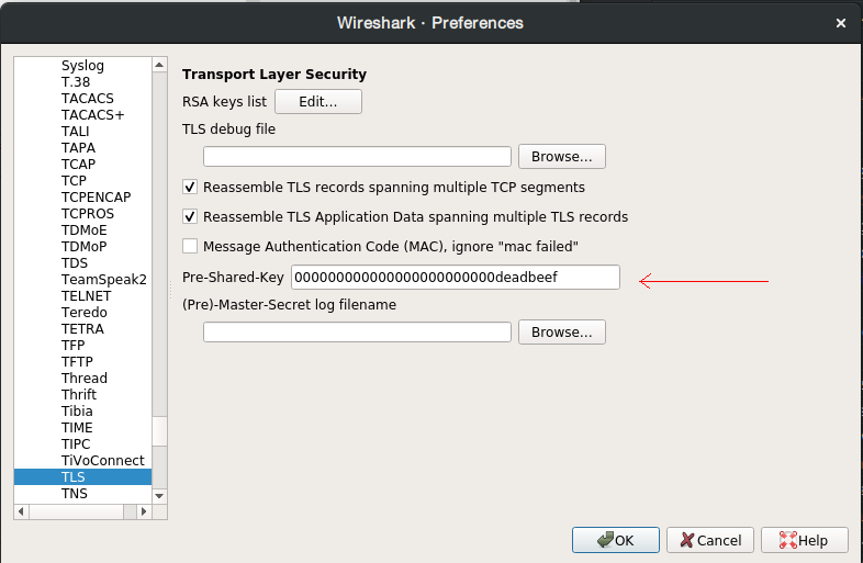
We are then able to see MQTT traffic as TLS payload.
MQTT over TLS with the ESP32 and Mongoose-OS
Mongoose-OS has a built-in MQTT client supporting TLS. This allows us to authenticate the server, but also the server infrastructure is able to authenticate the identity of incoming connections, that is, to validate that they belong to authorized users.
For further information on the MQTT client and using it without TLS, read this article. For more information on TLS, read this one.
Configuration
We’ll configure the ESP32 running Mongoose-OS to use the MQTT client and connect to a WiFi network. Since we are going to connect to a server (the MQTT broker), this is perhaps the simplest and fastest way to run our tests. This action can be done manually using RPCs (Remote Procedural Calls), writing a JSON config file, or it can be defined in the YAML file that describes how the project will be built. We’ve chosen this last option for our tests.
libs:
  - origin: https://github.com/mongoose-os-libs/mqtt  # Include the MQTT client
config_schema:
  - ["mqtt.enable", true]            # Enable the MQTT client
  - ["mqtt.server", "address:port"]  # Broker IP address (and port)
  - ["mqtt.ssl_ca_cert", "ca.crt"]   # Broker certificate, required
  - ["mqtt.ssl_cert", "sandboxclient.crt"]  # our certificate, for mutual authentication
  - ["mqtt.ssl_key", "sandboxclient.key"]   # our key, for mutual authentication
The most common port for MQTT over TLS is 8883. The broker can also ask us to send a username and password, full configuration details are available at the corresponding Mongoose-OS doc page. Finally, it is the broker who decides which type of authentication to use (one- or two-way), though we must provide our certificate when the broker asks for it.
Operation
Before we build our project and execute our code, it is perhaps convenient to have an MQTT client connected to the broker, so we can see the message the device will send at connect time. We’ve used a broker we installed in a server in our lab and connected to it with no authentication, so all we’ve shown in the MQTT article is valid here too.
After the code is compiled and linked (mos build) and the microcontroller’s flash is programmed (mos flash) using mos tool, we’ll watch the log and check if everything is going on as it should, or catch any possible errors. Remember we need to configure the proper access credentials to connect to our WiFi network of choice (SSID and password), and the address and port for the MQTT broker we are going to use. At the end of this note we show how to configure a Mosquitto broker.
One-way authentication
This way we can authenticate the server, that is, we can trust it is the one to whom we want to connect, but the server has no idea who can we be.
This is the simplest configuration and we only have to provide the CA certificate filename in the parameter ssl_ca_cert, the certificate has to be stored in the fs directory. This indicates the broker has to be validated.
[Mar 31 17:21:18.360] mgos_mqtt_conn.c:435    MQTT0 connecting to 192.168.5.3:8883
[Mar 31 17:21:18.585] mongoose.c:4906         0x3ffca41c ciphersuite: TLS-ECDHE-RSA-WITH-AES-128-GCM-SHA256
[Mar 31 17:21:20.404] mgos_mqtt_conn.c:188    MQTT0 TCP connect ok (0)
[Mar 31 17:21:20.414] mgos_mqtt_conn.c:235    MQTT0 CONNACK 0
[Mar 31 17:21:20.423] init.js:34              MQTT connected
[Mar 31 17:21:20.437] init.js:26              Published:OK topic:/this/test/esp32_807A98 msg:CONNECTED!
Two-way (mutual) authentication
This way we can authenticate the server and the client, that is, now the server knows we should be the one who our certificate says we are. This dual process requires lots of processing and we’ll notice that connection establishment takes longer. In this configuration we must provide our certificate and key in the fs directory, and configure parameters ssl_cert and ssl_key appropriately; otherwise the broker might give us a clue in its log, as Mosquitto does:
Mar 31 17:30:52 Server mosquitto[2694]: OpenSSL Error: error:140890C7:SSL routines:ssl3_get_client_certificate:peer did not return a certificate
Brokers: Mosquitto
These are minimal configurations for Mosquitto, take them as a quick help and not as a reference. Paths are in GNU/Linux form and we should put our certificates there.
One-way authentication (broker authentication)
listener 8883 192.168.5.1
log_dest syslog
cafile /etc/mosquitto/certs/ca.crt
certfile /etc/mosquitto/certs/server.crt
keyfile /etc/mosquitto/certs/server.key
Mutual (two-way) authentication
listener 8883 192.168.5.1
log_dest syslog
cafile /etc/mosquitto/certs/ca.crt
certfile /etc/mosquitto/certs/server.crt
keyfile /etc/mosquitto/certs/server.key
require_certificate true
Example
Companion example code available in Github, here and here. We’ll also need server credentials, I left a set here so we can do this easily.
Timer expired, I think…
Quite often we have several ways to perform a task. Sometimes we choose based on personal taste or affinity, others there is a context that enforces certain rules that limit our safe choices.
When working with software timers, I usually choose to use an old scheme based on multiple independent timers that has found its way through the assembly languages of many different micros and has finally landed in C. Sometimes, due to 32-bits being available, I may choose to simply check the value of a counter. In both cases, each timer and the counter are decremented and incremented (respectively) in an interrupt handler.
This requires that (in C) we declare this variable volatile so the compiler knows that this variable might change at any time without the compiler taking action in the surrounding code. Otherwise, loops waiting on this variable will be optimized out.
extern volatile uint32_t tickcounter;On the other hand, and due to the same reason, the access to this variable must be atomic, that is, it has to occur in a single processor instruction (or a non-interruptible sequence of them). Otherwise, the processor might accept an interrupt request in the middle of the instruction sequence that is reading the individual bytes forming this variable, and if this interrupt modifies this variable we would end up with an incorrect value. This happens, for example, if we use 32-bit counters/timers on most 8-bit micros; more info on this subject in another post.
Once we solve this issues, then there is the problem of counter length, the number of bits defining integer word size for our timers.
My timer scheme above is quite simple: each timer is decremented if it has a non-zero value, so to use one of this I simply write a value and then poll until I get a zero. There is obviously a jitter as there is a time gap from the moment I write the timer till it’s decremented by the interrupt handler, and another one since the timer reaches zero and the application reads the value.
However, reading a counter, on the other hand, poses some issues; and their solutions were the inspiration to write this post. Because of atomicity, we might end up being forced to use a small variable, a short length counter that will overflow in a short time.
What happens when this counter overflows ? Well, maybe nothing happens, if we take precautionary measures.
Everything will work as a charm and all tests will pass as long as the counter doesn’t overflow between readings, that is, counter length is enough for the application lifetime. For example, a 32-bit seconds counter takes 136 years to overflow. However a 16-bit milliseconds counter overflows every minute and fraction (65536 milliseconds).
If the time between counter readings is larger, there is the possibility that the counter may overflow more than once between checks. In this situation, we must use an auxiliary resource, as the counter alone can’t do it.
If, however, we can be sure that the counter will overflow at most once between checks, we just need to write proper code in order for our comparison to survive this overflow. Otherwise, as we’ve already said, everything will work fine most of the time, but “sometimes” (every time there is a counter overflow) we’ll get a glitch.
For the sake of this analysis, let’s consider the following scheme, we are using uppercase names in violation of some coding styles but we do it for counter highlight’s sake:
extern volatile uint32_t MS_TIMER;
uint32_t interval = 5000; // milliseconds
uint32_t last_time;
The following code snippets work fine, as the difference survives counter overflow and can be correctly compared to our desired value:
	last_time = MS_TIMER;

	if(MS_TIMER - last_time > interval)
	    printf("Timer expired\n");

	if(MS_TIMER - interval > last_time)
	    printf("Timer expired\n");
On the other hand, this does not work properly
uint32_t deadline;

	/* I must not do this
	deadline = MS_TIMER + interval;
	if(MS_TIMER > deadline)
	    printf("Timer expired\n");
	*/
If, let’s say, MS_TIMER is 0xF8000000 and interval is 0x10000000, then deadline will be 0x08000000 and MS_TIMER is clearly larger than deadline from the beginning, this causes the timer to expire immediately (and that is not what we want…).
A workaround is to use signed integers, and this works with time intervals up to MAXINT32 units:
int32_t deadline;
int32_t interval = 5000; // milliseconds

	deadline = MS_TIMER + interval;
	if((int32_t)(MS_TIMER - deadline) > 0)
	    printf("Timer expired\n");
To dive into more creative ways might result in timers that never expire when the counter is higher than MAXINT32, as this is seen as a negative number and so smaller than any desired time (that is a positive number); but do work when our device is started or reset. These can be considered as errors when choosing counter length (including sign).
As we’ve seen, some problems show themselves when referring to a time that is MAXINT32 time units after the system starts. This is usually 2^31, and this, for a milliseconds counter, is around 25 days; and for a seconds counter about 68 years. There can be several errors lurking deeply inside some Linux (and other Un*x-like) systems that will surface once they need to make reference to a time after year 2038 (the seconds counter starts at the beginning of year 1970).
If, on the other hand, we use 16- or 8-bit schemas…
In these examples we used ‘greater than’ in comparisons; this guarantees that the time interval will be longer than requested. If, for example, we set it right now and ask for a one second interval, and one millisecond later the interrupt handler increments the counter, should we use a ‘greater than or equal’ comparison our timer will expire immediately (well, in 1ms…). Also, if we set it 1ms after the interrupt took place it will expire in 1,999s instead of 1s. In a scenario where increment and comparison are not asynchronous, we can avoid jitter and use a ‘greater than or equal’ comparison.
MSP430
Escribí este texto por allá por el 2003… no recuerdo haberlo corregido, puede tener desde inconsistencias y errores hasta horrores ortosemantácticos. Lo dejo aquí por si a alguien le resulta útil o el ejército de buscadores lo atrae al resto del contenido, que debe ser al menos unos casi veinte años mejor.
Introducción
La serie MSP430 de Texas Instruments es un conjunto de microcontroladores RISC de 16 bits de ultra bajo consumo, con una serie de periféricos sumamente interesantes, interconectados en un mapa de memoria lineal con arquitectura Von Neumann, es decir, buses integrados de direcciones y datos para instrucciones y datos. Tanto RAM como flash, SFRs (Special Function Registers, registros para funciones especiales) y periféricos son direccionados por un único bus de direcciones y entregan sus datos en un único bus de datos; ambos internos. Un sistema de reloj altamente flexible permite que el procesador pueda elegir la frecuencia de operación de la CPU y de diversos periféricos de entre las opciones de clocking disponibles, minimizando el consumo cuando no se requiere la operación de alguno.
Características principales
- Arquitectura de ultra-bajo consumo
- Retención de datos en memoria RAM interna con un consumo de 0,1 uA
- Operación como reloj de tiempo real con un consumo promedio estimado de 0,8uA
- Consumo en estado activo promedio de 250uA, a una velocidad de operación de 1 MIPS (un millón de instrucciones por segundo)
- Conversores analógico-digitales de 10 ó 12 bits, de 200Ksps (doscientas mil muestras por segundo), con sensor de temperatura y generador de tensión de referencia integrados
- Conversores digital-analógicos de 12 bits
- Temporizadores (timers) comandados por un comparador interno, permiten medir elementos resistivos
- Supervisión de la tensión de alimentación
- CPU de 16 bits, RISC (Reduced Instruction Set Code)
- Gran cantidad de registros, de modo de eliminar cuellos de botella
- Set de instrucciones optimizado para programación de alto nivel
- Sólo 27 instrucciones y 7 modos de direccionamiento
- Interrupciones vectorizadas
- Programación en sistema de la memoria flash interna; permitiendo flexibilidad para la actualización del código y captura de datos (data logging)
El consumo del chip en el estado inactivo es del orden de 1uA. El consumo en estado activo, con una tensión de alimentación de 3V, y con un clock de 1MHz, es de aproximadamente 250uA. El MSP430 puede pasar de un estado al otro en un máximo de 6us, permitiendo que el programador mantenga un consumo extremadamente bajo y a la vez sea capaz de atender una interrupción en un tiempo sumamente pequeño.
Todos los periféricos del chip han sido optimizados para lograr un máximo control sobre el consumo del sistema, su funcionamiento es independiente del estado de la CPU, por lo cual es posible mantener un timer con funciones de RTC (Real Time Clock, reloj de tiempo real), para la ejecución de tareas periódicas, mientras el chip consume cerca de 1 µA. También es posible esperar el pulsado de una tecla, datos de un port serie, o realizar la tarea de refresco de un display LCD mientras la CPU duerme. Poseen un estado adicional en el cual son capaces de retener los datos en registros y RAM con un consumo de 0,1 µA, de este estado sólo es posible salir a través de una interrupción externa o reset, ya que ninguno de los clocks está operativo.
Sistema de clocking
El sistema de relojes ha sido diseñado expresamente para aplicaciones con alimentación a baterías. Posee un reloj auxiliar (ACLK), que puede funcionar directamente con un cristal de 32KHz (ideal para aplicaciones de RTC) o con un cristal de alta frecuencia, agregando los capacitores correspondientes. Posee además un oscilador controlado digitalmente (DCO, Digitally Controlled Oscillator) de alta velocidad, que puede proveer el reloj maestro (MCLK) para la CPU y los periféricos más rápidos y/u otro reloj adicional (SMCLK) para otros periféricos. Las características de diseño de este DCO garantizan que esté activo y estable en menos de 6us luego de su inicio, de modo que las soluciones basadas en MSP430 puedan aprovechar al máximo las características de alta performance de la CPU utilizando su procesamiento en ráfagas cortas, como por ejemplo la atención de eventos por interrupciones.
Algunos modelos incluyen un segundo oscilador de alta frecuencia para aumentar las opciones de clocking disponibles.
En resumen, tenemos básicamente tres fuentes de reloj: ACLK, MCLK y SMCLK. ACLK toma reloj del oscilador a cristal; MCLK y SMCLK derivan su reloj de un oscilador a cristal o del DCO, a elección del programador. Es posible intercalar un divisor (prescaler) para bajar la frecuencia de reloj en cada una de ellas. La CPU toma reloj de MCLK, y los diversos periféricos incorporan opciones para seleccionar la fuente de reloj y algunos incluyen, a su vez, otros divisores. Todos los osciladores pueden ser prendidos y apagados a voluntad, para minimizar el consumo, y la CPU puede “desconectar” su fuente de reloj, para pasar a los estados de bajo consumo.
CPU
La CPU del MSP430 es un RISC de 16 bits. El direccionamiento de memoria es lineal (no existen bancos ni paginado ni segmentado de ningún tipo) y puede hacerse por bytes o por words. El acceso por words requiere que éstas estén alineadas, es decir, comenzando en una dirección par. La figura a la izquierda muestra el mapa de memoria, donde se aprecia la integración de RAM, flash, SFRs y periféricos en un mismo espacio de direccionamiento lineal.
El set de instrucciones es altamente ortogonal; con muy pocas excepciones todas las instrucciones pueden utilizarse en todos los registros con cualquier modo de direccionamiento. Esto resulta una amplia ventaja sobre otras arquitecturas anunciadas como RISC pero que necesitan de un registro especial que es operando forzado de todas las operaciones, al igual que el acumulador en la mayoría de los CISC. En el MSP430, cualquier registro es fuente y cualquiera es destino, para cualquier modo de direccionamiento, excepto el modo indirecto, que sólo puede ser empleado para el operando fuente.
Dada la reducida cantidad de instrucciones, resulta sumamente fácil y rápido el aprendizaje. Dada la gran cantidad de modos de direccionamiento, el programador se dedica a resolver su algoritmo en vez de luchar contra la arquitectura de la CPU.
El código generado es sumamente compacto, y compite con otros procesadores de 8 bits de similares características. A la hora de comparar, debe tenerse en cuenta que si bien las instrucciones y datos en el MSP430 son de 16 bits, la flexibilidad de la arquitectura generalmente permite realizar la tarea deseada con menos instrucciones. Para portar una aplicación desarrollada en un CISC a la arquitectura del MSP430 y poder relizar una comparación, es muy probable que se deba re-escribir el código pensándolo de forma diferente y haciendo uso de conceptos que le son más propios. Por ejemplo, es muy común en muchos CISC y algunos pseudo-RISC el utilizar instrucciones de tipo “prueba y salto” (test and branch), es decir, chequear un flag en una dirección de memoria o registro y saltar si está activo. En el MSP430, es muchísimo más efectivo utilizar un esquema más parecido a una máquina de estados, es decir, utilizar “bytes de estado” (status bytes), que guardan el estado actual. El salto a una u otra parte del código se realiza simplemente sumando esa variable o registro al Program Counter (PC).
Para aquellos de nosotros acostumbrados a algunas instrucciones comunes en los CISC, el assembler del MSP430 emula algunas instrucciones aceptando el mnemónico y generando código RISC equivalente, por ejemplo: para desplazar a la izquierda un registro, algunos CISC incorporan una instrucción como por ejemplo RLA (rotate left aritmetically, rotar a la izquierda insertando ceros por la derecha), siendo que ya la tienen, dado que sumar un registro a sí mismo constituye una multiplicación por dos y en aritmética binaria eso es lo mismo que desplazar el registro a la izquierda. Por este motivo, el assembler del MSP430 acepta la instrucción RLA <operando> y genera el código ADD <operando>,<operando>.
El set de registros está compuesto por 16 registros, de éstos, cuatro son utilizados como PC (program counter), SP (Stack Pointer), SR (Status Register, parte baja de R2) y CG (Constant Generator, parte alta de R2 y todo R3), los restantes 12 registros pueden usarse como acumuladores o punteros de uso general definidos por el usuario. Puede observarse la potencialidad de esta arquitectura extremadamente versátil, de gran poder de cálculo y que resulta muy eficiente para ser programada en lenguaje C, o bien para lograr un programa bien estructurado. El CG utiliza el par R2/R3, que emula mediante modos de direccionamiento algunas constantes de uso típico, como 0, 1, -1, etc, evitando, de este modo, la necesidad de utilizar una palabra de 16 bits para esta constante. Por ejemplo, la instrucción CLR <operando> es reemplazada en primera instancia por el assembler por el código MOV #0, <operando>. Analizando el código de máquina, vemos que su estructura (desglose de los campos de operando fuente y destino, y modo de direccionamiento fuente y destino) corresponde a la siguiente instrucción: MOV R3, <operando>. La utilización del registro R3 en modo de direccionamiento de registros como operando fuente, indica que el CG contiene el valor 0. Este es un concepto muy complejo que veremos en más detalle al analizar la CPU; la idea de exponerlo aquí es mostrar cómo es posible economizar espacio de memoria de programa.
Programación, escritura y depuración del código (debugging)
Los MSP430 pueden programarse y accederse mediante una interfaz JTAG. Existen notas de aplicación de Texas Instruments en las cuales pueden apreciarse circuitos de aplicación (SLAA149).
Además, incorporan una ROM con un programa interno que permite que el microcontrolador pueda recibir paquetes de un formato especial y programar la memoria interna. Esta particularidad se denomina “bootstrap loader” y utiliza algunos recursos del procesador, que si bien pueden reusarse para otras aplicaciones, deberán ser tenidos en cuenta. La ejecución del código en esta ROM comienza cuando el procesador detecta una secuencia especial en un par de pines, al momento de reset. Existen notas de aplicación de Texas Instruments en las cuales se indica el hardware necesario para aprovechar esta característica especial (SLAA096).
De este modo, es posible, con mínimo hardware, disponer de una interfaz para realizar programación y actualización del programa en circuito, es decir, sin necesidad de retirar los micros de la placa.
Por supuesto que, además de ésto, el fabricante ofrece herramientas de desarrollo y programación. Los FET (Flash Emulation Tool) son herramientas que permiten grabar el dispositivo y trabajar sobre el sistema. Si bien su costo es bastante bajo, dada la disponibilidad de soluciones abiertas en la forma de notas de aplicación, y a su espíritu constructor, dichas herramientas no han sido evaluadas por el autor. El circuito esuqemático de varios FET está disponible en la página web de Texas Instruments, con lo cual es posible construírse una económica interfaz JTAG para port paralelo de PC que permite programar y depurar paso a paso.
El entorno de desarrollo “oficial”, al momento de escribir este documento, es el IAR Embedded Workbench de IAR Systems, obtenible en forma gratuita de la página web de Texas Instruments. Se trata de una versión especial que provee el compilador C, pero limitado a generar 1K de código objeto como máximo. Esto no resulta en disminución alguna para los amantes del assembler, que encuentran en éste un agradable entorno de desarrollo; pudiendo trabajar de forma modular, ya que el proyecto tiene su definición, los archivos involucrados, y el proceso de ensamblado y/o compilado es seguido por un linkeado que maneja el tema de la relocalización. Por supuesto que quienes así lo deseen pueden optar por comprar la versión que viene con el FET, o la versión completa sin restricciones para el compilador.
Entre las opciones open source, existe un port del tradicional GCC, disponible en la Internet, que nos permite compilar ANSI C sin restricciones.
Memoria
Encontramos memoria RAM y flash ó ROM, según el modelo. La dirección de inicio de la flash/ROM depende de la cantidad presente en el chip, de modo que la dirección final siempre sea 0FFFFh, para poder almacenar los vectores de interrupción y reset sin necesidad de incorporar un bloque adicional de flash, como hacen otros microcontroladores. Para el caso de memoria flash, la misma se halla segmentada en bloques de generalmente 512 bytes, la escritura puede hacerse por byte o por word, pero el borrado es por bloque. Generalmente también incluyen dos segmentos adicionales de 128 bytes, destinados al alojamiento de datos de calibración, de modo de poder aprovechar todos los segmentos principales para código y tablas. La operación sobre la flash puede hacerse en cualquier momento, el micro incluye un sistema de autocontención que lo demora si intenta acceder a una posición que está siendo escrita o borrada, por lo que no es estrictamente necesario disponer de código de borrado/escritura en RAM, las rutinas de borrado y grabación pueden residir en la misma flash, con la salvedad de que estén en un segmento diferente al que es objeto de la operación. Actualmente, la flash soporta unos 100.000 ciclos de borrado.
En cuanto a la RAM, siempre comienza en 0200h, aunque la cantidad total depende de cada dispositivo.
Ambos tipos de memoria pueden utilizarse indistintamente para código o datos, y pueden ser accedidas como words o como bytes, siempre respetando la alineación: los bytes pueden estar en direcciones pares o impares; las words sólo pueden residir en locaciones pares. La parte baja (byte menos significativo) de una word está siempre en la dirección par, seguida por la parte alta en la dirección inmediata superior. Por ejemplo, si una word reside en xxx4h, la parte baja está en xxx4h y la parte alta en xxx5h. Una misma variable o espacio puede accederse de una u otra forma, a criterio y conveniencia del programador, siempre que se respete la alineación. Supongamos que en la posición 0204h está guardado el dato 02123h:
MOV 0204h, R5 ; Lee word presente en posición de memoria 0204h y lo guarda en R5: R5=02123h
MOV.B 0204h, R6 ; Lee byte presente en posición de memoria 0204h y lo guarda en R6: R6=023h
MOV.B 0205h, R7 ; Lee byte presente en posición de memoria 0205h y lo guarda en R7: R7=021h
Leer un byte y leer un word alineado requiere el mismo tiempo de CPU, al contrario de otros micros de 16 o más bits, y por supuesto que los de 8 bits.
Periféricos y SFRs
Los periféricos de 16 bits mapean en el área de 0100h a 01FFh, y deben ser accedidos utilizando instrucciones de acceso por words, es decir, leyendo los 16 bits de una sola vez. Si se intenta accederlos por bytes, solamente se podrán acceder las direcciones pares, el byte más significativo (situado, como dijéramos, en la dirección impar subsiguiente) se leerá como cero.
Los periféricos de 8 bits mapean en el área de 010h a 0FFh, y deben ser accedidos usando acceso por bytes. El uso de direccionamiento por words para acceder a estos dispositivos puede resultar en datos incorrectos en el byte más significativo (dirección impar).
Algunas funciones particulares están configuradas por Registros de Funciones Especiales (SFRs), organizados por bytes en los primeros 16 bytes del espacio de memoria (00 a 0Fh). Deben ser accedidos solamente mediante acceso por bytes. Estos registros controlan la operación y configuración del microcontrolador.
El contenido y variedad de los periféricos, así como la función de los SFRs dependen de cada modelo de microcontrolador en particular. Particularmente, es destacable el hecho de que no sólo hay coincidencias en diversos miembros de una misma familia, sino que por lo general, aún en miembros de distintas familias puede observarse que el mismo periférico suele ocupar la misma posición de memoria y hasta el mismo pin de conexión; contrariamente a muchos otros microcontroladores de otras marcas.
Documentación
La hoja de datos de cada dispositivo o grupo de dispositivos tiene características eléctricas propias del mismo, el seteo de los SFRs que le son propios, y alguna descripción particular de algún periférico que le es propio.
En general, la descripción de cada uno de los periféricos y el seteo de los registros asociados, se encuentra en el manual del usuario de la familia correspondiente, junto con el set de instrucciones y la descripción de la CPU. Esto evita mantener información redundante en las hojas de datos, que resultan simples y concisas en vez de largamente extensas como sucede con otros fabricantes, que incluyen toda la información en cada hoja de datos. La redundancia se encuentra entre familias, es decir, las guías del usuario de diversas familias tienen información redundante entre sí. Por ejemplo, si un desarrollador trabaja con la familia 1xx, como es el caso de quien escribe, le basta con tener la guía o manual del usuario de la familia 1xx y las hojas de datos de cada dispositivo que usa: 11×1, 11×2/12×2, 12x, 13x/14x, por ejemplo.
On atoms and clocks
Interrupts, as their name implies, may interrupt the program flow of a microprocessor at any point, any time, even though sometimes they seem to intentionally do it in the most harmful way possible. The very reason of their existence is to allow the processor to handle events when it is not convenient to be waiting for them to happen or regularly poll for their status, or to handle those types of events requiring a fast and low latency attention.
When carefully utilized, interrupts are a powerful ally, we can even build multiple-task schemes assigning an independent periodic interrupt to each task.
When haphazardly used, interrupts may bring more problems than solutions; in particular, we can’t share variables or subroutines without taking due precautionary measures regarding accessibility, atomicity, and reentrability.
An interrupt may occur at any point in time, and if it occurs in the middle of a multi-byte variable update it can (and in fact it does) wreak havoc on other tasks. These may hold “partially altered” values that in the real world are incorrect values, and probably dangerously incoherent for the software. A typical and frequently forgotten example are timing or date and time variables. The main program happily takes these variables byte by byte in order to show them on the display screen, without thinking that, if they are updated by an interrupt, these are not restricted to being handled before or after our action and not in the middle of it. If those values are only shown at the display screen there is no further inconvenience, correct values will be shown one second later, but if they are logged or reported, we’ll be in serious trouble explaining why there is a record with a date almost a year off, as in the following example:

Some time ago there was this microcontroller-oriented developing environment that in order to “solve this inconvenience” introduced the concept of ‘shared variables’. Every time one of these variables was accessed or changed, the compiler introduced a set of instructions to disable the interrupts during this action and enable them back at the end. The problem I find on these strategies is that this is very bad educationally speaking, as bad as protection diodes in GPIOs (commented in this article): the user does not understand what is going on, does not know, doesn’t learn. Furthermore, frequent accesses to these variables produce frequent interrupt disables, which translate to latency jitter in interrupt handling.
Even though in the case of a multi-byte variable as the one in the example this is quite evident, the same happens with a 32- or 16-bit variable on 8-bit micros that do not have proper instructions to handle 32-bit (most of them) or 16-bit entities. Atomicity, that is, the ability to access the variable as an indivisible unit, is lost, and when accesses to these variables are shared by asynchronous tasks, there is the possibility of superimposing those accesses and then ending with something like what we’ve seen in the example above.
If our C development environment has signal.h, then we should find in there a definition for the sig_atomic_t type, that identifies a variable size that can be accessed atomically. Otherwise, and as a recommendation in these environments, the user must know the processor being used and act accordingly.
In multiprocessing environments there are other issues, that we will not list here.
Corollary
An interrupt may occur at any point in time, as long as it is enabled. The probability of this happening just in the very moment we are accessing a multi-byte variable in a non-atomic way is pretty low, particularly if it is a brief, non frequent access, that is not synchronized to interrupts. However, this probability is greater than zero, and so, given enough repetitions, it is likely to occur. Leaving the correct behavior of a device to the Poisson distribution function should not be considered a good design practice…
This post contains excerpts from the book “El Camino del Conejo“ (The way of the Rabbit), translated with consent and permission from the author.